What are errors?
When we make a measurement, we can never be sure that it is 100% "correct". All devices, ranging from a simple ruler to the experiments at CERN, have a limit in their ability to determine a physical quantity.
Error analysis attempts to quantify this in a meaningful way. Error analysis allows us to ask meaningful questions on the quality of the data, these include
- Do the results agree with theory?
- Are they reproducible?
- Has a new phenomenon or effect been observed?
It should be noted that in Physics the words "error" and "uncertainty" are used almost interchangeably. This is not ideal, but get used to it! In reality, “error” refers to the difference between the quoted result and the accepted/true value being measured while “uncertainty” refers to the range of values your result could take given the capabilities of your equipment. See more on this here.
Accuracy and Precision
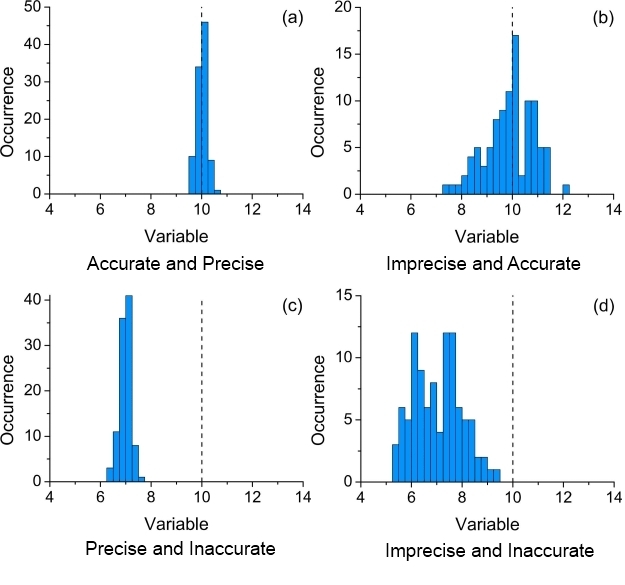
These are two terms that have very different meanings in experimental physics. We need to be able to distinguish between an accurate measurement and a precise measurement. An accurate measurement is one in which the results of the experiment are in agreement with the ‘accepted’ value. Note this only applies to experiments where this is the goal – measuring the speed of light, for example. A precise measurement is one that we can make to a large number of decimal places.

Fig 1. Diagrams illustrating the differences between accuracy and precision
Types of Errors
We need to identify the following types of errors
- Systematic errors - these influence the accuracy of a result
- Random errors - these influence precision
- Mistakes - bad data points.
It should be noted that “human error” is not a thing in physics and data analysis! These are what you would refer to as “mistakes”, which are generally not reported in technical documents and should be avoided altogether.
Systematic Errors
Introduction
Systematic errors are a constant bias that are introduced into all your results. Unlike random errors, which can be reduced by repeated measurements, systematic errors are much more difficult to combat and cannot be detected by statistical means. They cause the measured quantity to be shifted away from the 'true' value.
Dealing with systematic errors
When you design an experiment, you should design it in a way so as to minimise systematic errors. For example, when measuring electric fields you might surround the experiment with a conductor to keep out unwanted fields. You should also calibrate your instruments, that is use them to measure a known quantity. This will help tell you the magnitude of any remaining systematic errors.
A Famous Systematic Error
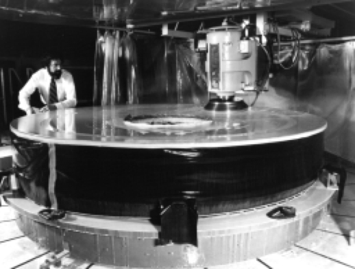
One famous unchecked systematic error towards the end of the 20th century was the incorrect grinding of the Hubble Space telescope's main mirror (shown in Fig. 2) resulting in an unacceptable level of spherical aberration. The mirror was perfectly ground, but to the wrong curve. This led to the sacrifice of an instrument in order to fit corrective optics into the telescope on the first Shuttle maintenance mission (STS-61) to the orbiting observatory.
Importantly, this episode illustrates that although some simple systematic errors can be corrected after data has been collected others need new data and hardware to compensate for failings in experimental design.

Fig. 2 The Hubble main mirror at the start of its grinding in 1979.
Random Errors – Measurement Uncertainty
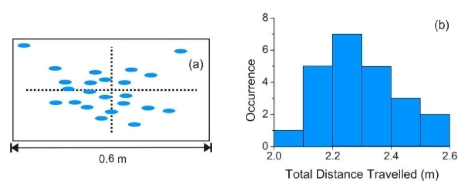
Minimising random errors is a primary concern of experimental physics. Random errors are harder to control and manifest as the scattering of repeat measurements over a range (as seen in Fig.3). More random error leads to lower precision. It should be noted that repeated measurements are not always the best solution. Recommending repeat measurements should be justified, and averaging poor quality data will not necessarily give a good quality result.

Fig. 3: The range of a ball-bearing launched from a spring-loaded projectile launcher. Repetition of the experiment with the same conditions yields different results. Therefore, there is an error related to this quantity.
When analysing data, the standard error is a measure of that set’s random error. When taking individual measurements, however, the random error can be quantified in the uncertainty on each measurement. There are two simple rules to follow, which in most cases will be true. Above all else, use your best judgement about the uncertainty of your measurements. If a digital reading is fluctuating wildly or the analogue scale is hard to read, make sure your recorded error reflects that.
Analogue Devices
If your measuring device has an analogue scale (e.g. rulers, vernier scales etc) then the error is ± half the smallest increment
For example, take the ruler in Fig. 4, the error on this instrument is ±0.5 mm (using the metric scale).

Fig 4. An image of a ruler
Digital Devices
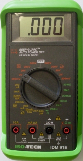
If your measuring device has a digital scale (e.g. multimeters) then the error is ± 1 unit of the lowest significant figure
For example, take the image of the multimeter shown in Fig. 5, the error in the measurement would be ±0.001 V.

Fig 5. An image of a multimeter
Error Analysis
In Physics, we often combine multiple variables into a single quantity. The question is, how do we calculate the error in this new quantity from the errors in the initial variables?
There are two main approaches to solving this: the functional approach and the calculus approximation.
The following information applies to single variable functions only. For information on multi-variable functions, see Measurements and their Uncertainties by I.G. Hughes and T.P.A. Hase (OUP, 2010)
Functional Approach
This approach simply states that the error on the final result Z will be the function’s value including the error minus the function’s value without. In other words, if we have a function of the from Z = f(A), where f is a general function, then it follows that

Where
- Alpha Z is the error on Z
- A bar is the mean of A
- Alpha A is the standard error on A
In most circumstances, we assume that the error on A is symmetrical. However, this is not always true and sometimes the error bars in the positive and negative directions are different sizes.
Calculus Approximation
From the functional approach, we can make a calculus-based approximation for the error. This is done by considering a Taylor series expansion of equation 1. Assuming αA is small relative to the mean of A, we can deduce equation 2.

If we recall that Z = f(A), then equation 3 follows from a substitution of equation 2 into equation 1.

It should be stressed that this equation is only valid for small errors. However, in most cases this is valid and so the calculus approximation is a good way to propagate errors.
Another important point to note is that the calculus approach is only useful when the differential is solvable. With non-trivial functions such as Z = arcsin(A) the functional approach would be more useful.


/prod01/prodbucket01/media/durham-university/departments-/physics/teaching-labs/VT2A9034-1998X733.jpeg)